Creating and Exercising a Custom Single Degree of Freedom System
Note
You can download this example as a Python script: custom-sdof-system.py or Jupyter notebook: custom-sdof-system.ipynb.
Creating a new system
The first step is to import a “blank” SingleDoFLinearSystem and initialize
it.
from resonance.linear_systems import SingleDoFLinearSystem
msd_sys = SingleDoFLinearSystem()
Now define the constant variables for the system. In this case, the single degree of freedom system will be described by its mass, natural frequency, and damping ratio.
msd_sys.constants['m'] = 1.0 # kg
msd_sys.constants['fn'] = 1.0 # Hz
msd_sys.constants['zeta'] = 0.1 # unitless
msd_sys.constants
{'m': 1.0, 'fn': 1.0, 'zeta': 0.1}
Define the coordinate and speed. The software assumes that the speed is defined as the time derivative of the coordinate, i.e. \(v = \dot{x}\).
msd_sys.coordinates['x'] = 1.0 # m
msd_sys.speeds['v'] = 0.0 # m/s
msd_sys.coordinates
{'x': 1.0}
msd_sys.speeds
{'v': 0.0}
msd_sys.states
{'x': 1.0, 'v': 0.0}
Now that the coordinate, speed, and constants are defined the equations of motion can be defined. For a single degree of freedom system a Python function must be defined that uses the system’s constants to compute the coefficients to the canonical second order equation, \(m \dot{v} + c v + k x = 0\).
The inputs to the function are the constants. The variable names should match those defined above on the system.
import numpy as np
def calculate_canonical_coefficients(m, fn, zeta):
"""Returns the system's mass, damping, and stiffness coefficients given
the system's constants."""
wn = 2*np.pi*fn
k = m*wn**2
c = zeta*2*wn*m
return m, c, k
msd_sys.canonical_coeffs_func = calculate_canonical_coefficients
Once this function is defined and added to the system \(m,c,k\) can be computed using:
msd_sys.canonical_coefficients()
(1.0, 1.2566370614359172, 39.47841760435743)
The period of the natural frequency can be computed with:
msd_sys.period()
1.005037815259212
All information about the system can be displayed:
msd_sys
System name: SingleDoFLinearSystem
Canonical coefficients function defined: True
Configuration plot function defined: False
Configuration update function defined: False
Constants
=========
m = 1.00000
fn = 1.00000
zeta = 0.10000
Coordinates
===========
x = 1.00000
Speeds
======
v = d(x)/dt = 0.00000
Measurements
============
Simulating the free response
The free_response() function simulates the now fully defined system given
as an initial value problem. One or both of the coordinates and speeds must be
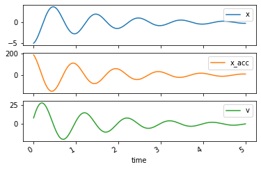
set to provide a free response. The following shows the response to both
\(x\) and \(v\) being set to some initial values.
msd_sys.coordinates['x'] = -5.0
msd_sys.speeds['v'] = 8.0
free_response() returns a Pandas DataFrame with the time values as the
index and columns for the coordinate, speed, and additionally the time
derivative of the speed (acceleration in this case). See
https://pandas.pydata.org/pandas-docs/stable/getting_started/dsintro.html for
an introduction to DataFrame.
trajectories = msd_sys.free_response(5.0)
trajectories
| x | x_acc | v | |
|---|---|---|---|
| time | |||
| 0.00 | -5.000000 | 187.338992 | 8.000000 |
| 0.01 | -4.910728 | 181.496514 | 9.844723 |
| 0.02 | -4.803311 | 175.015195 | 11.627801 |
| 0.03 | -4.678398 | 167.928429 | 13.343009 |
| 0.04 | -4.536697 | 160.271570 | 14.984469 |
| ... | ... | ... | ... |
| 4.96 | -0.217071 | 8.839775 | -0.214970 |
| 4.97 | -0.218780 | 8.796369 | -0.126761 |
| 4.98 | -0.219609 | 8.719006 | -0.039156 |
| 4.99 | -0.219566 | 8.608415 | 0.047509 |
| 5.00 | -0.218663 | 8.465444 | 0.132905 |
501 rows × 3 columns
There are a variety of plotting methods associated with the DataFrame that
can be used to quickly plot the trajectories of the coordinate, speed, and
acceleration. See more about plotting DataFrames at
https://pandas.pydata.org/pandas-docs/stable/user_guide/visualization.html.
axes = trajectories.plot(subplots=True)
Response to change in constants
This system is parameterized by its mass, natural frequency, and damping ratio. It can be useful to plot the trajectories of position for different values of \(\zeta\) for example.
Set the initial conditions back to simply stretching the spring 1 meter:
msd_sys.coordinates['x'] = 1.0
msd_sys.speeds['v'] = 0.0
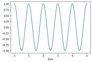
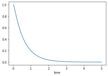
Now change \(\zeta\) to different values and simulate the free response to see the different damping regimes:
Un-damped, \(\zeta=0\)
msd_sys.constants['zeta'] = 0.0 # Unitless
trajectories = msd_sys.free_response(5.0)
axes = trajectories['x'].plot()
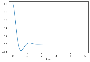
Under-damped, \(0<\zeta<1\)
msd_sys.constants['zeta'] = 0.5 # Unitless
trajectories = msd_sys.free_response(5.0)
axes = trajectories['x'].plot()
Critically damped, \(\zeta=1\)
msd_sys.constants['zeta'] = 1.0 # Unitless
trajectories = msd_sys.free_response(5.0)
axes = trajectories['x'].plot()
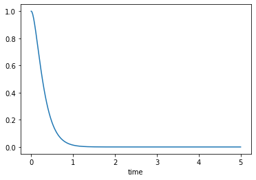
Over-damped, \(\zeta>1\)
msd_sys.constants['zeta'] = 2.0 # Unitless
trajectories = msd_sys.free_response(5.0)
axes = trajectories['x'].plot()
Adding measurements
It is often useful to calculate the trajectories of other quantities. Systems
in resonance allow “measurements” to be defined. These measurements are
functions of the constants, coordinates, speeds, and/or time. To create a new
measurement, create a function that returns the quantity of interest. Here a
measurement function is defined that calculates the kinetic energy
(\(\frac{1}{2}mv^2\)) of the system and then added to the system with
variable name KE.
def calculate_kinetic_energy(m, v):
return m*v**2/2
msd_sys.add_measurement('KE', calculate_kinetic_energy)
Once added, the measurement will be computed and added to the DataFrame
containing the trajectories:
msd_sys.constants['zeta'] = 0.5 # Unitless
trajectories = msd_sys.free_response(5.0)
trajectories
| x | x_acc | v | KE | |
|---|---|---|---|---|
| time | ||||
| 0.00 | 1.000000e+00 | -39.478418 | 8.881784e-16 | 3.944305e-31 |
| 0.01 | 9.980674e-01 | -36.999522 | -3.823857e-01 | 7.310941e-02 |
| 0.02 | 9.924348e-01 | -34.530060 | -7.400220e-01 | 2.738162e-01 |
| 0.03 | 9.833490e-01 | -32.078904 | -1.073048e+00 | 5.757160e-01 |
| 0.04 | 9.710551e-01 | -29.654314 | -1.381689e+00 | 9.545318e-01 |
| ... | ... | ... | ... | ... |
| 4.96 | 4.648115e-08 | 0.000006 | -1.189485e-06 | 7.074377e-13 |
| 4.97 | 3.487003e-08 | 0.000006 | -1.132570e-06 | 6.413573e-13 |
| 4.98 | 2.383263e-08 | 0.000006 | -1.074788e-06 | 5.775850e-13 |
| 4.99 | 1.337624e-08 | 0.000006 | -1.016414e-06 | 5.165491e-13 |
| 5.00 | 3.505453e-09 | 0.000006 | -9.577074e-07 | 4.586018e-13 |
501 rows × 4 columns
and can be plotted like any other column:
axes = trajectories['KE'].plot()
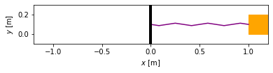
Plotting the configuration
resonance systems can plot and animate at the system’s configuration. To do
so, a custom function that generates a configuration plot using matplotlib must
be defined and associated with the system. Below a plot is created to show an
orange block representing the mass and a spring attached to the block. The
spring() function conveniently provides the x and y data needed to plot the
spring.
import matplotlib.pyplot as plt
from resonance.functions import spring
# create a new constant to describe the block's dimension, l
msd_sys.constants['l'] = 0.2 # m
def create_configuration_figure(x, l):
# create a figure with one or more axes
fig, ax = plt.subplots()
# the `spring()` function creates the x and y data for plotting a simple
# spring
spring_x_data, spring_y_data = spring(0.0, x, l/2, l/2, l/8, n=3)
lines = ax.plot(spring_x_data, spring_y_data, color='purple')
spring_line = lines[0]
# add a square that represents the mass
square = plt.Rectangle((x, 0.0), width=l, height=l, color='orange')
ax.add_patch(square)
# add a vertical line representing the spring's attachment point
ax.axvline(0.0, linewidth=4.0, color='black')
# set axis limits and aspect ratio such that the entire motion will appear
ax.set_ylim((-l/2, 3*l/2))
ax.set_xlim((-np.abs(x) - l, np.abs(x) + l))
ax.set_aspect('equal')
ax.set_xlabel('$x$ [m]')
ax.set_ylabel('$y$ [m]')
# this function must return the figure as the first item
# but you also may return any number of objects that you'd like to have
# access to modify, e.g. for an animation update
return fig, ax, spring_line, square
# associate the function with the system
msd_sys.config_plot_func = create_configuration_figure
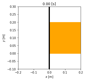
Now the configuration plot can be generated with plot_configuration(). This
returns the same results as the function defined above.
fig, ax, spring_line, square = msd_sys.plot_configuration()
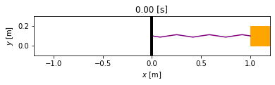
Animating the configuration
Reset to un-damped motion and simulate again
msd_sys.constants['zeta'] = 0.1
trajectories = msd_sys.free_response(5.0)
To animate the configuration, create a function that updates the various
matplotlib objects using any constants, coordinates, speeds, and/or the special
variable time. The last input arguments to this function must be all of the
extra outputs of plot_configuration() (excluding the figure which is the
first output). The order of these must match the order of the
plot_configuration() outputs.
def update_configuration(x, l, time, # any variables you need for updating
ax, spring_line, square): # returned items from plot_configuration() in same order
ax.set_title('{:1.2f} [s]'.format(time))
xs, ys = spring(0.0, x, l/2, l/2, l/8, n=3)
spring_line.set_data(xs, ys)
square.set_xy((x, 0.0))
msd_sys.config_plot_update_func = update_configuration
Now that the update function is associated, animate_configuration() will
create the animation. Here the frames-per-second are set to an explicit value.
animation = msd_sys.animate_configuration(fps=30)
If using the notebook interactively with %matplotlib widget set, the
animation above will play. But animate_configuration() returns a matplotlib
FuncAnimation object which has other options that allow the generation of
different formats, see
https://matplotlib.org/api/_as_gen/matplotlib.animation.FuncAnimation.html for
options. One option is to create a Javascript/HTML versions that displays
nicely in the notebook with different play options:
from IPython.display import HTML
HTML(animation.to_jshtml(fps=30))
Response to sinusoidal forcing
The response to a sinusoidal forcing input, i.e.:
can be simulated with sinusoidal_forcing_response(). This works the same as
free_response except it requires a forcing amplitude and frequency.
msd_sys.coordinates['x'] = 0.0 # m
msd_sys.speeds['v'] = 0.0 # m/s
Fo = 10.0
omega = 2*np.pi*3.0 # rad/s
forced_trajectory = msd_sys.sinusoidal_forcing_response(Fo, omega, 5.0)
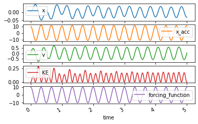
Note that there is now a forcing_function column. This is the applied
forcing function.
forced_trajectory
| x | x_acc | v | KE | forcing_function | |
|---|---|---|---|---|---|
| time | |||||
| 0.00 | 0.000000 | 10.000000 | 6.938894e-18 | 2.407412e-35 | 10.000000 |
| 0.01 | 0.000496 | 9.679225 | 9.871978e-02 | 4.872797e-03 | 9.822873 |
| 0.02 | 0.001957 | 8.978820 | 1.923176e-01 | 1.849302e-02 | 9.297765 |
| 0.03 | 0.004313 | 7.924765 | 2.771159e-01 | 3.839662e-02 | 8.443279 |
| 0.04 | 0.007459 | 6.555691 | 3.497615e-01 | 6.116656e-02 | 7.289686 |
| ... | ... | ... | ... | ... | ... |
| 4.96 | -0.023218 | 8.674053 | -3.722232e-01 | 6.927505e-02 | 7.289686 |
| 4.97 | -0.026486 | 9.839976 | -2.793765e-01 | 3.902562e-02 | 8.443279 |
| 4.98 | -0.028773 | 10.655573 | -1.765928e-01 | 1.559251e-02 | 9.297765 |
| 4.99 | -0.029997 | 11.091961 | -6.753058e-02 | 2.280189e-03 | 9.822873 |
| 5.00 | -0.030115 | 11.133696 | 4.392935e-02 | 9.648938e-04 | 10.000000 |
501 rows × 5 columns
The trajectories can be plotted and animated as above:
axes = forced_trajectory.plot(subplots=True)
fps = 30
animation = msd_sys.animate_configuration(fps=fps)
HTML(animation.to_jshtml(fps=fps))
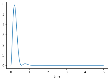
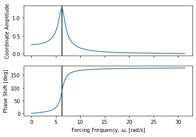
Frequency response
The frequency response to sinusoidal forcing at different frequencies can be
plotted with frequency_response_plot() for a specific forcing amplitude.
axes = msd_sys.frequency_response_plot(Fo)
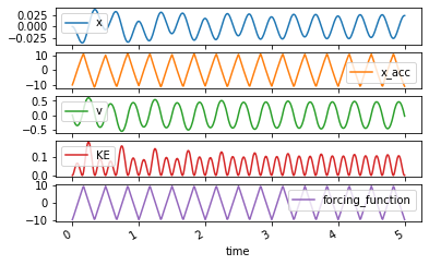
Response to periodic forcing
Any periodic forcing function can be applied given the Fourier series coefficients of the approximating function. The following function calculates the Fourier series coefficients for a “sawtooth” shaped periodic input.
def sawtooth_fourier_coeffs(A, N):
"""
A : sawtooth amplitude, Newtons
T : sawtooth period, seconds
N : number of Fourier series terms
"""
n = np.arange(1, N+1)
an = A*(8*(-1)**n - 8) / 2 / np.pi**2 / n**2
return 0, an, np.zeros_like(an)
a0, an, bn = sawtooth_fourier_coeffs(Fo, 20)
These coefficients can be provided to periodic_forcing_response() to
simulate the response:
wb = 2*np.pi*3.0 # rad/s
trajectory = msd_sys.periodic_forcing_response(a0, an, bn, wb, 5.0)
trajectory
| x | x_acc | v | KE | forcing_function | |
|---|---|---|---|---|---|
| time | |||||
| 0.00 | -3.469447e-18 | -9.797526 | -6.938894e-18 | 2.407412e-35 | -9.797526 |
| 0.01 | -4.773325e-04 | -8.653652 | -9.344627e-02 | 4.366102e-03 | -8.789924 |
| 0.02 | -1.821290e-03 | -7.332725 | -1.731808e-01 | 1.499579e-02 | -7.622252 |
| 0.03 | -3.896544e-03 | -5.927083 | -2.395012e-01 | 2.868041e-02 | -6.381879 |
| 0.04 | -6.565825e-03 | -4.583400 | -2.921305e-01 | 4.267012e-02 | -5.209711 |
| ... | ... | ... | ... | ... | ... |
| 4.96 | 1.860597e-02 | -6.335998 | 3.117475e-01 | 4.859327e-02 | -5.209711 |
| 4.97 | 2.138612e-02 | -7.530659 | 2.423054e-01 | 2.935596e-02 | -6.381879 |
| 4.98 | 2.341220e-02 | -8.748665 | 1.608547e-01 | 1.293711e-02 | -7.622252 |
| 4.99 | 2.456569e-02 | -9.845257 | 6.805327e-02 | 2.315623e-03 | -8.789924 |
| 5.00 | 2.473372e-02 | -10.728694 | -3.603302e-02 | 6.491893e-04 | -9.797526 |
501 rows × 5 columns
axes = trajectory.plot(subplots=True)
fps = 30
animation = msd_sys.animate_configuration(fps=fps)

HTML(animation.to_jshtml(fps=fps))